We often ask whether some event, like a merger announcement, dividend omission, or stock split, has an impact on stock prices. Since we have CRSP data available, it is pretty easy to construct a test to answer this question. In general the idea is simple; first determine what a "normal" return ought to be for the stock in question, and then see whether the actual return during the "event window" is more or less than this "normal" return. Of course the devil is in the details: What is a "normal" return? Over what time period do you determine this "normal" return? How long is the event window? Are there characteristics of reported stock returns that make these measurements unreliable? I'm not going to answer all of these questions for this problem set. You'll get some answers in your seminar. Instead, I'm going to focus on how to construct some of the more basic tests so you can get experience programming them.
All of this can be done in SAS--albeit with some difficulty. I think it is easier to do it in Fortran, if you know enough Fortran. Over the semester we'll look at both ways.
You should read "Using Daily Stock Returns; The Case of Event Studies" by Stephen J. Brown and Jerold B. Warner in Journal of Financial Economics Volume 14, Issue 1 (March, 1985) pages 3-31, and also "Valuation Effects of Security Offerings and the Issuance Process" by Wayne H. Mikkelson and Meghan Partch in Journal of Financial Economics Volume 15, Issue 1 (March 1986) pp. 31-60. I have a master that you can use to make copies.
Event date--the date the event occured
Event window--several days before and after the event. This is the
time period over which you think you will observe some market reaction to the event.
We use some days before the event because lots of time news leaks out before the
public announcement. We use some days after the event because sometimes it takes a
day or two for the market to fully impound the effects of the event into the stock price.
Event time--trading days relative to the event date. Usually the
event date is considered day 0 and days before the event date are negative. So day
-5 is 5 days before the event, day +5 is 5 days after the event.
Normal return--the return you would expect on the stock during the event
window if there had been no event.
Abnormal return--the actual stock return less the predicted normal
return.
We have daily and monthly returns available. If you really want, you can construct other interval returns--weekly, two-weekly, annual, etc. Since most of the events we look at are of short duration you will usually use daily, or at most weekly, returns. For these exercises we'll use daily returns.
There are at least three ways to identify a "normal" return.
We won't talk about the pros and cons of these methods here. You will get some of that in your seminar. Once you have determined what is a normal return, the abnormal return is just the actual return minus the predicted normal return. We'll estimate the first three measures.
You can estimate the normal return before, during, or after the event. For the purposes of our exercises we will use days -104 to -5 for the estimation period. We'll use days -4 to +1 for the event window.
There are a number of ways to test for significance, depending on how you characterized normal above. I'll specify a test for each of your exercises.
Identifying abnormal returns is usually easier in a portfolio than in individual stocks. For that reason the tests will be on portfolios of stocks rather than on individual stocks.
Brown and Warner used the following test statistics for the null hypothesis that excess returns are zero. These tests assume you are testing a collection of firms' abnormal returns.
Let Ai,t be firm i's abnormal return (either mean adjusted, market adjusted,
or market model adjusted) on day t.
Let Abart be the mean (over all the companies in the sample) abnormal return on
day t.
Let s be the
standard deviation of the Abart over all days in the estimation period (using
N-1 weighting, so it is an estimate of the population standard deviation).
The test statistic for a given mean (over all the companies) abnormal return on a given
day, Abart, is
T = Abart/s
If enough days are in the estimation period--over 200, then the statistic is assumed to be normal. Otherwise it is Student-t.
Let SAbar be the
sum of the average abnormal returns during the event window.
Since s is the
estimate of the standard deviation of one day's abnormal return, sn1/2
is an estimate of the standard deviation of the sum of n independant abnormal returns.
The test statistic is
z = SAbar/(sn1/2 )
and is assumed to be unit normal. n is the number of days in the event window.
Mikkelson and Partch only use market model abnormal returns so Ai,t = Ri,t - (alpha + beta RM,t )--they call these prediction errors, PE (We'll still use the Abar terminology). On day t, Abart is calculated just as above--the mean abnormal return over all firms on day t.
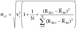
The difference between Mikkleson and Partch's test statistic, and that of Brown and Warner, is in how the expected standard deviation of abnormal returns is calculated and the fact that they allow for different numbers of days in the event window for each firm. Mikkleson and Partch allow for each calendar day's abnormal return to have a different standard deviation. So corresponding to each abnormal return Ai,t is a standard deviation si,t calculated as follows:
Let vi2 be the variance of the residual from firm i's market model regression (the one you used to find alpha and beta). Assume you used N observations in this regression (i.e. N days in the estimation period) then:
is the standard deviation of each day t's abnormal return for company i, where the RM with the bar over it is the mean market return over the N-day estimation period. Note that this will differ for each firm because the average of the market return is over different days, unless of course some of the firms share the same event date.
Then the standardized prediction errors for each day and each company,
SPEi,t = Ai,t /si,t
should all be Student-t with variance N/(N-2).
For a given day, the average of these prediction errors over all the firms in the sample (there are M firms in the sample), ASPEt is approximately normal with variance 1/(# firms in sample) = 1/M. This gives us the test statistic for an abnormal return on a given day, t, as
Zt = M1/2 (ASPEt)Under the null hypothesis, Zt is distributed unit normal.
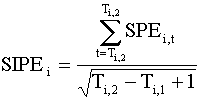
Sometimes you want to test whether the abnormal performance over a number of days is zero--like Brown and Warner did above. This just means having an event window that is longer than one day. But suppose you have different length event windows for different companies? Company A's event window might be days -3 to +2, company B's might be days -5 to +2. To aggregate all these potentially different-length event windows you need to create a different variable for each company such that they are all distributed the same. So if for company i the event window runs from Ti,1 to Ti,2 then first calculate the standardized interval prediction error for company i, SIPEi , as
Then just average all of these across all of the firms and normalize by multiplying by M1/2 to get the test statistic:
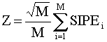
which should be asymptotically unit normal.
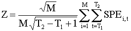
Note: If all of the event windows are the same length and cover the same (event-time) days,T1 to T2 , then this test statistic just becomes:
My results:
Just for comparison, my results for the first couple of days during the estimation period for the exercise above are:
CALENDAR LOADED. 9943 DAYS IN CALENDAR - (19620702-20011231)
n-ew = 100
alpha-ew = -1.757551567E-3
beta-ew = 0.769114435
stdres-ew = 8.181140758E-3
SASs RMSE = 8.264199831E-3
n-vw = 100
alpha-vw = -7.125223638E-4
beta-vw = 0.829781473
stdres-vw = 7.093603257E-3
SASs RMSE-vw = 7.1656215E-3
time comp-per mktadjew mktadjvw mmadjew mmadjvw ret
ewretd
-104 0.00043 0.01064 0.01256 0.01005 0.01121 0.00047
-0.01018
-103 0.00698 0.01831 0.01858 0.01746 0.01733 0.00702
-0.01129
-102 -0.00701 -0.00200 -0.00084 -0.00139 -0.00117 -0.00697 -0.00497
-101 -0.00332 -0.00082 0.00186 0.00037 0.00170 -0.00328 -0.00246
-100 0.00184 -0.00197 -0.00022 0.00068 0.00085 0.00188
0.00384
-99 -0.00238 -0.00542 -0.00221 -0.00295 -0.00152 -0.00234 0.00307
-98 0.00560 0.00817 0.00891 0.00934 0.00907
0.00564 -0.00253
-97 0.00557 0.00043 0.00020 0.00338 0.00184
0.00561 0.00518
The program you wrote for IBM in assignment 1 can be used for a bunch of companies. Write a loop around your program above to:
Permno and event data data for assignment 2:
Permno Event date
12060 19880421
80718 19820212
88322 19870623
88306 19871113
77002 19940713
79084 19941010
85013 19980623
34826 19840506